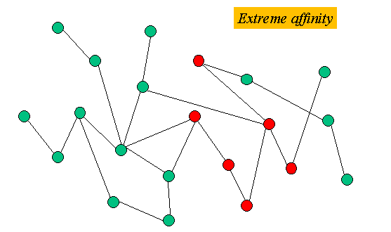
Figure 1: Nodes close to each other have a positive affinity relationship.
This web page is a summary of our paper and an outline of basic affinity concepts. We have also put together a brief slide presentation highlighting our findings. This research is part of the Denali Project funded by the NSF ITR Program.
For any network or graph, consider a subset S of nodes. Affinity describes the clusteredness or closeness of S. Nodes with high affinity are very close to each other. We use terms such as clustered, positive affinity, and positive attraction synonymously.

Figure 1: Nodes close to each other have a positive affinity relationship.
Nodes with high disaffinity are very far apart from each other. We use terms such as declustered, negative affinity, and negative attraction synonymously.
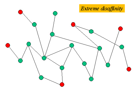
Figure 2: Nodes far apart from each other have a negative affinity relationship.
Affinity is relevant to many applications. For example, imagine a web conference transmission, in which a single source in New York were communicating to multiple receivers in San Francisco. Rather than being randomly distributed throughout the network, those receivers would be clustered at a few points in the network. As another example, imagine a sensor network study, in which a scientist were measuring temperature readings from distant points on an island. Again, rather than being randomly distributed, the source transmitter nodes would be declustered throughout the island. It is also possible to combine affinity and disaffinity in the same scenario: for example, node clusters that have strong disaffinity with the other clusters.
As the above examples show, affinity is a realistic consideration for many network studies. Thus, several questions come to mind:
Phillips, Shenker and Tangmunarunkit (2000) developed a probabilistic selection algorithm that has been used in several studies. The probability of any node joining S is a function of its distance to the nearest node already in S. Let ρi be the probability of selecting node i. Note that Σ ρi must equal 1. Below are two examples of affinity selection.
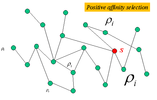
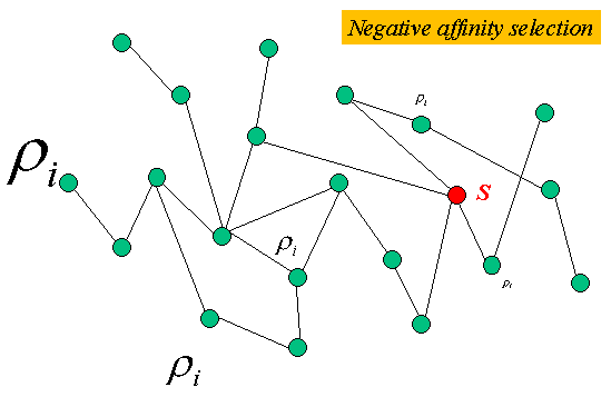
To explain the algorithm in a bit more detail, the formula for ρi is:

In our paper, we propose several affinity analysis metrics. Prior to our work, studies had compared affinity performance using the input parameter β. We show how affinity metrics i) provide a better characterization of actual affinity, ii) are stronger predictors of network performance, and iii) necessary when analyzing a pre-existing subset of nodes.
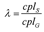
The metric we choose for presentation in our paper is λ. If cplG is the characteristic path length of the network (average path length among all paths), and cplS is the characteristic path length of S, then define λ as:
The paper discusses the benefits of and reasoning behind choosing λ.
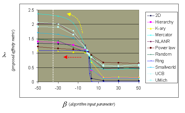
In Figure 5, we plot λ versus β. As the dotted white line shows, the actual affinity level varies for a constant value of β depending on the network topology. Moreover, the red and yellow arrows indicate that affinity bounds differ across networks. Some networks permit a wide range of affinity levels for S, while others allow only a limited variation of affinity. It is not just number of nodes and edges that affect affinity variation; so too do network density and overall topology. Our paper discusses network topology effects in more detail.
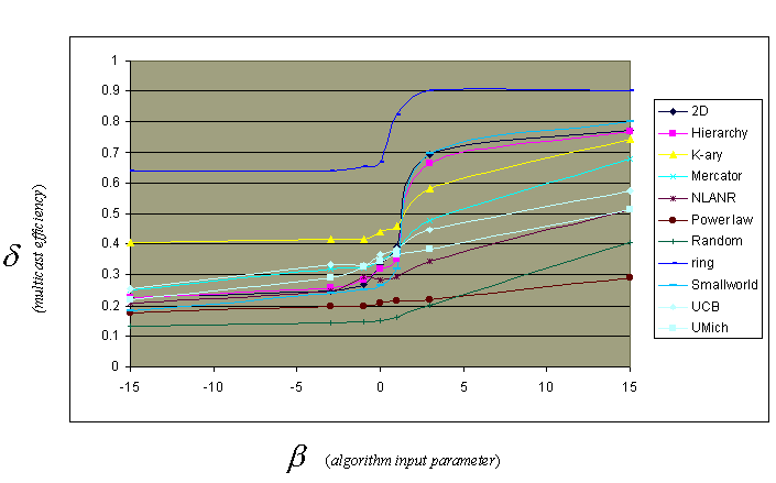
We perform three case studies (multicast, replica placement, and sensor networks) and show that in each case, the actual affinity level of S is a better predictor of network performance than is the value of the input parameter used to generate S. In other words, it's better to classify subsets of nodes by their actual affinity λ, rather than by β. Figures 6 and 7 demonstrate this finding for the multicast case. We observe a much better linear fit with λ; in the paper, we present regression results. δ is a multicast efficiency metric defined by Chang, Govindan, Jamin, and Shenker.
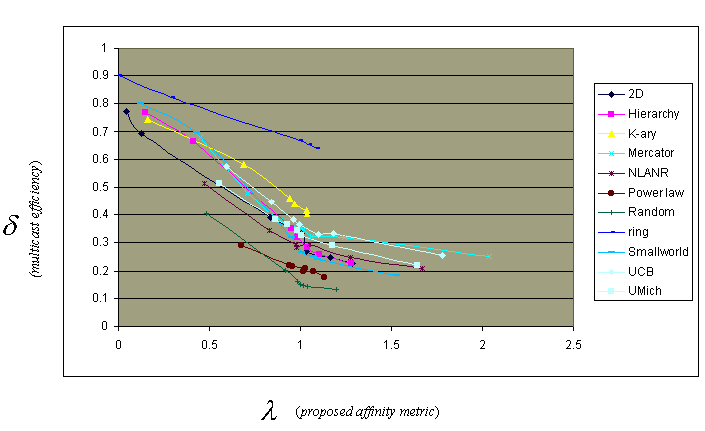
Figure 6: δ versus λ for the multicast case study.
To learn more about affinity, please read our paper.